Determining Pressure Drop for Control Valve Sizing

Pressure drop must be determined when sizing control valves for a particular system.

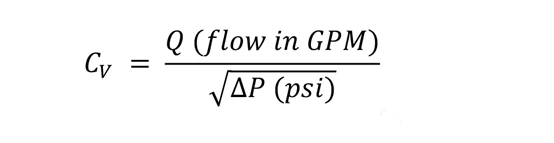
Most people familiar with control valves have seen the formula for calculating the valve capacity (Cv) required to flow through a given amount of water (or liquid of similar density):

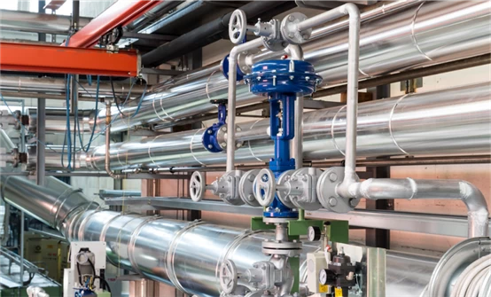
Pressure drop of control valve

A plumbing system exists to perform the useful functions of the facility. It could be cooling a product stream, conveying ingredients, refilling buckets or hundreds of other functions. Typically, once an operator or engineer understands the required function and load range of the system, the minimum and maximum flow rates required to perform this function can be determined. Alternatively, if a single design condition is known, a reasonable guess at the expected flow range can provide minimum and maximum flow values ​​for valve sizing.

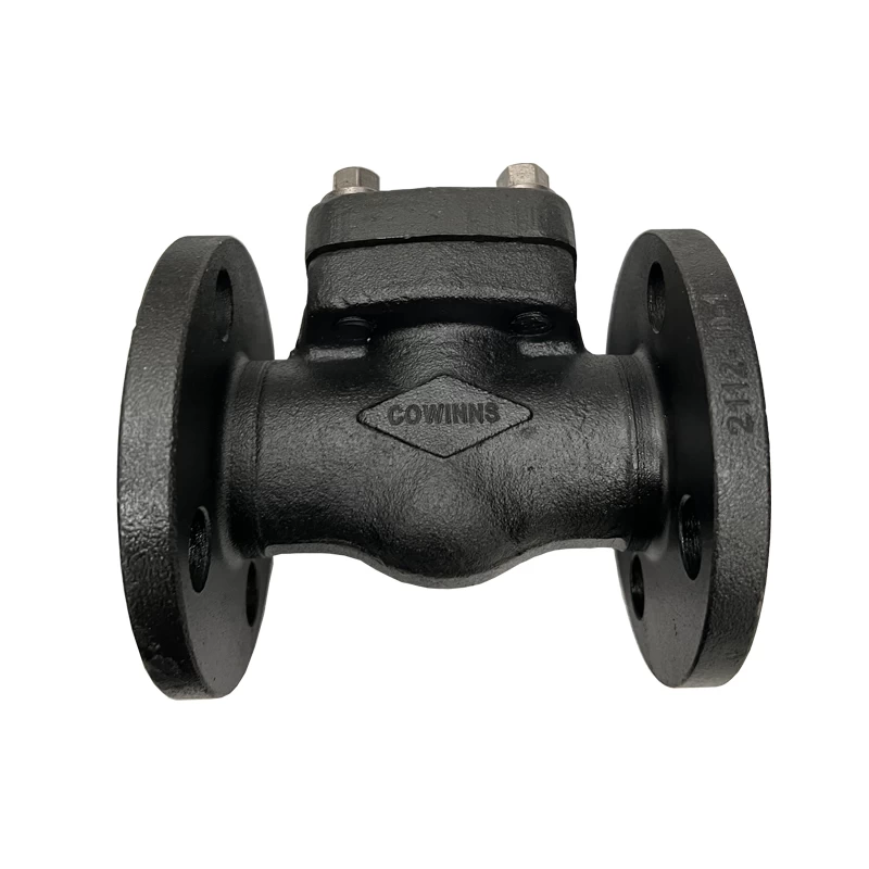
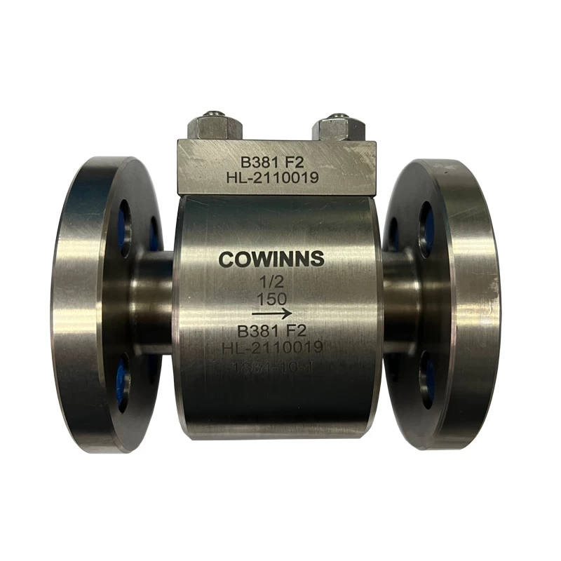
"Almost" all components of the plumbing system are fixed. These components include pipes, fittings, filters or screens, isolation valves and heat exchangers. And also high pressure check valve. The pressure loss in each of these assemblies varies with the flow rate of the fluid flowing therethrough. Once the process engineer has determined the minimum and maximum flow rates, the pressure losses in these stationary components can be calculated for each flow rate.

Note that the word "almost" is used above. This is because one component that is not secured is the control valve. The control system will adjust the control valve as needed so that the system provides the flow needed to perform its designed function. The portion of the overall system differential pressure that is not consumed by stationary components in the system must appear across the control valve.

Calculation

There is a calculation program that determines the differential pressure (ΔP) at the control valve for a given flow in the system. For each flow condition, start upstream of the valve at a known pressure location. A good example of this type of location is a centrifugal pump, where the pressure can be determined from the head curve. Subtract the pressure loss for each element from that point in the system. Using the calculated pressure loss at the minimum flow rate for each elbow, isolation valve, heat exchanger and other fixed equipment, proceed along the path of the system, deducting each pressure loss.

Once this is done, the system pressure upstream of the valve can be recorded as P1 under minimum flow conditions.

The next step is to calculate the pressure leaving control valve P2. Do this in a similar way to the first calculation, just in reverse. This means that a point downstream of the valve must be chosen with a known pressure. A good example is a jar with a known head. Another problem is that the stream is vented into the atmosphere. From this position, the pressure loss needs to increase until it reaches the outlet of the valve. The reason why these numbers are added rather than subtracted as in the previous example is because we are moving upstream in the pipeline rather than downstream. This result was recorded as P2 under minimum flow conditions.

Once these two numbers (P1 and P2) are recorded, the pressure drop that the control valve must account for can be easily determined using the following formula:

Repeat this process using the value determined by the maximum flow rate. If the upstream known pressure location is a fixed speed centrifugal pump, you need to slide right on the pressure-flow curve to the output head value for maximum flow, which will be lower than the head value for minimum flow. At maximum flow, the pressure loss per fixture will be greater, so the slope of the system pressure graph will be steeper than at minimum flow conditions. See Figure 1 for an example of a piping system pressure map.

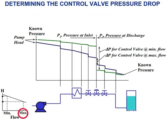
Figure 1. Determining control valve pressure drop

Once P1 for maximum flow is determined, start at a point downstream of the known pressure and work in reverse, again using the higher value of pressure loss caused by the higher maximum flow. This will give you P2 at maximum flow conditions.

Understanding System Pressure Loss

As shown in Figure 1, in a typical piping system, the value of ΔP at minimum flow conditions is greater than that at maximum flow conditions.

If one were to graph P1 and P2 for the total flow that the system can provide, a graph such as the one shown in Figure 2 for a typical example could be generated.

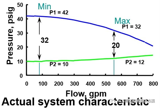
Figure 2 Pressure curve or system characteristics.

The top line shows the value of P1, which will start at a higher value and decrease as the flow increases. The lower line on the graph (the value of P2) will start at a relatively low value and increase as the flow increases. At any flow value, the distance between these two lines is the valve size differential pressure, ΔP. This graph is sometimes called a pressure curve. It can also be viewed as a proxy for system characteristics - a summary of specific piping system characteristics similar to those inherent in control valves.

Once the exact values for P1, P2 and ΔP are determined, the (Cv) calculation and control valve selection can be done easily and accurately.

Conclusion

The bottom line is that when sizing a control valve for a particular system, there is no way to estimate or assume what the pressure drop will be. Calculations must be made based on the nature of the system, taking into account all fixed components in a given system and how that system will operate at minimum and maximum flow rates.